Simulation of Obstacle Avoiding Autonomous Robots Controlled by Neuro-Evolution
Wolfgang Wagner
wolfgang.wagner@iname.com
1999
Introduction
Lots of research is currently being done in the development of control
systems for autonomous robots [Links]. The basic capability
of these robots is to walk around in an unknown environment and to fulfil
various tasks (e.g. avoiding obstacles) without the presence of any human
remote control. They could be used in different fields, like acting in
dangerous environments, cleaning waste pipes, exploring other planets and
many more.
It is easy for human beings or even insects to act autonomously in
known or unknown environments, but for computer controlled robots it is
still a great challenge. Although the requirements are easy to define the
capability of reacting to unexpected situations requires complex algorithms
and data structures.
One way to implement client control systems is to take living creatures
as a model and to use neural nets (NNs) like our brain. Artificial neural
nets (ANNs) have already proved to be a useful and flexible mechanism for
controlling different kinds of technical devices [Ri94].
But knowing their structure, and the capability of simulating their behavior
on a computer is not enough. Like in real life they have to learn in order
to solve problems. Although the way how living creatures (or in fact
their brains) learn has not been completely investigated, several learning
strategies for ANNs have already been developed. One of these strategies
is neuro-evolution (NE) . It uses the evolutionary algorithm that was developed
from the results of the exploration of natural evolution and applies it
to ANNs. Although the combination of NNs and evolution does not exist in
nature, it has already been proved to be a useful learning strategy for
ANNs.
The following paper describes a computer simulation that allows one
to verify that NE can be used for the breeding of control systems of autonomous
robots.
Just to be Precise
In the following chapters the expression 'robot' is used whenever the robot's
control system is meant; just like in every days life we don't speak about
someone's brain if we mean someone. In the chapter about the genetic algorithm
the term robot is replaced by creature because it better matches the other
terms concerning genetic evolution.
robot's control system <- robot <- creature.
The Simulation
In order to test the capability of NE for the development of robot's control
systems, simulated robots and a simulated environment in which they can
move around have to be defined. The environment has to be somehow hostile
for robots in order to be able to distinguish between good and bad adapted
behavior.
Two tasks have been defined that our (simulated) robots have to meet.
They have to:
-
Avoid obstacles which are walking around controlled by a random walk algorithm.
-
Keep together in order to propagate.
These two demands force the robots to take decisions in different situations
depending on their current local environment. The capability to take the
right decision at the right moment is the fitness of the robot.
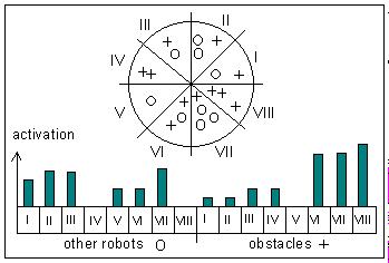
In order for robots to react to their environment some kind of sensor
interface has to be defined that gives a picture of the local environment.
These sensors are defined by the following rules:
The robot can distinguish between other robots and obstacles. It can
determine the distance of each of these objects within a certain scope.
Objects which are out of scope cannot be recognized. The local environment
of robots is divided into octants. In each of these octants the number
of other robots is counted and weighted by the distance of the particular
object. The same is done for obstacles. This leads to a vector of 16 values,
which represents the distribution of robots and obstacles around a robot.
In addition to the sensors, there has to be an effectors interface that
allows one to control the movements of the robots. This interface is composed
of the steer heading of the robot and of its velocity. The steer heading
can be set to a value between 0 and 7 where 0 means 0 o, 1 means
45 o, 2 means 90o , ... 7 means 315o.
The velocity can be set between 0 and a maximum value of 50 pixels per
simulation step. Any value within this range can be chosen, independent
of the current value.
With the definition of the sensor - and the effector interface we can
imagine a control system (that does not necessarily have to be an ANN)
which guides the movements of a robot according to the values of the sensor
interface.
The Genetic Algorithm
Genetic algorithms can be seen as search algorithms that can be used to
find nearly optimal solutions in arbitrarily formed search spaces. In natural
genetics this search space is the set of all combinations of DNA strings
of a certain species. An optimal DNA string (genotype) is one that creates
fit creatures (phenotypes). In order to ascertain which pheno- or genotype
is fitter than others, they have to be comparable in a certain way. In
real life they are compared by the capability of their phenotypes to survive
and to propagate. Creatures well adapted to their environment will live
longer and will by that have a greater chance of meeting partners than
poorly adapted ones. If two creatures meet each other they can propagate,
where the genotype of the children by crossing over the parents genes.
Applying repeated crossover to a final population creates relatively
identical genotypes in a short period of time. This would be the end of
progress for the evolutionary process, and even worse; a population like
this would loose the ability to adapt to a changing environment. To always
ensure a certain variance of behavior inside a population there has to
be a mechanism to change the genotype randomly. Variance is introduced
through gene mutation.
The above described rules lead to the simple genetic algorithm [Go89
] witch consists of three key operations.
-
Selection
-
Crossover
-
Mutation
These general rules where implemented in our simulation in the following
way: To start the genetic algorithm we have to generate a hostile environment
for our creatures. This is done by adding obstacles that walk around controlled
by a random walk algorithm. Then the simulation is initialized with a certain
amount of creatures. As the parameters for these "first generation creatures"
are random values, the result is a kind of random walk. Whenever one of
them touches an obstacle it dies immediately. These conditions result in
a population of very quickly dying creatures. If the number of creatures
is less than a minimum, new "random creatures" are generated. For a certain
amount of time the simulation remains in the state of just generating "random
creatures" which don't show any sensible. If a creature shows by chance
an environmentally adapted allowing it to survive long enough, and if at
the same time another one fulfils the same preconditions and if those two
manage to come somehow close together, the first crossover takes place.
E.g. the first child of the simulation is born.
This "birth" means that one or more (twins) new creatures are created
whose control systems are generated by applying the crossover and mutation
operation on the parents genotypes. If the creatures, generated by the
genetic operation, show the same, or an even better adaptation to their
environment as their parents, they also have the chance to produce children
in the same way as their parents did.
This creates a population of well behaving creatures after a relatively
short time. The number of creatures would explode if it was not limited
by an upper limit. If this limit is exceeded the whole population gets
temporarily infertile. Two creatures meet in this infertile period don't
get children even if all necessary conditions are fulfilled. If a creature
survives for a maximum time it dies because of old age. This natural death
lowers the population size and after a while the creatures get fertile
again.
Whenever a child is born, the mutation operation is applied to its
genotype. No mutation takes place during the lifetime of creatures.
The Artificial Neuronal Network (ANN)
In the above chapters the phenotype of creatures/robots was often mentioned
without an explanation of what this phenotype should be. One possible implementation
is with the use of an ANN. It has already been demonstrated that they have
the capability of controlling mobile robots [Links].
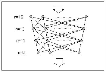
For this project a feed forward net with 4 layers was chosen. The input
layer consists of 16 and the output layer of 8 neurons. The in-between
layers have 11 and 13 neurons. Every neuron, except the neurons of the
input layer, is connected with every neuron of the previous layer with
one weighted connection. The structure of the connections is fixed. The
only parameters that can be varied are the weights of the connections.
The Neurons
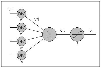
The net is built from neurons which are represented by a simple mathematically
model [Ri94]. Every neuron has an integer value representing
the degree of stimulation. This integer value can be in the interval (-a,
a) where 'a' has the value of 1000. Every connection between neurons contains
a weight also represented by an integer out of the interval (-b,
b) without 0. The value of 'b' is 100 in our net. The value of a neuron
is calculated in the following way: Given that the values of the preceding
neurons are calculated, the values of the input neurons are then preprocessed
by applying the weights of the corresponding synaptic connections using
the formula:
v1 = v0 DIV w
v1 ... pre-processed value
v0 ... value of the preceding neuron
w ... weight of the synaptic connection
Beware that using the DIV function results in a highly non-linear behavior
when forwarding activation to succeeding layers. It seems as if this non-linearity
has no negative consequences on the behavior of the net. If ratio of the
maximum value of weights (b) to the maximum value of stimulation (a) is
too large, we easily get into the situation where all values get pre-processed
to zero. The ratio of 100 to 1000 seems to be a good assumption for our
net. These pre-processed values are then summarized and evaluated by the
so called transfer function.
vs = T (SUM (v11 ... v1n))
v1i ... Pre-processed values of the synaptic connections
T ... Transfer function
As a transfer function the sigmoid function was chosen
v = a * (2 / (1 + EXP (-vs * s)) - 1)
a ... maximum value of stimulation
vs ... sum of pre-processed values
s ... constant stretch factor of the sigmoid function (0.01 in
our net)
Genetic Operations on ANNs
When working with ANNs to control our robots and using a genetic algorithm
to search for a nearly optimal control system, we have to define how to
apply the basic genetic operations (selection, crossover and mutation)
to the ANN. Selection does not have to be defined for ANNs separately,
as it is independent of the control system. Crossover and Mutation are
dependant on the structure of the control system.
Crossover
In nature, crossover is applied to (two) DNA strings each of which represents
a code containing all the properties of the corresponding creature. The
result is a new code from which a new creature is formed that has to prove
its fitness in its environment. Applying crossover to ANNs means finding
a code which contains the values of all parameters of the ANN so that we
can apply the crossover operation on it. The parameters of our ANN are
its weights since we have defined the structure to be constant. One possible
representation of the above mentioned code is a binary string. Mapping
the weights to a binary string is easy as the values are already integer
values. Defining an order to the weights and concatenating the binary represented
integer values generates automatically a binary string.
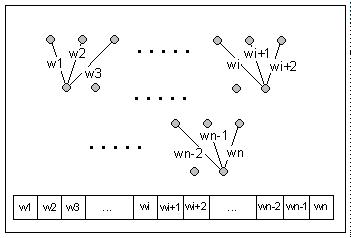
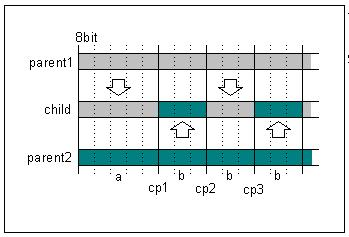
If you have (two) binary strings, created by the above mentioned mapping
algorithm the crossover operation can be applied to them to create a new
string from which a new ANN can be generated later. You start with one
of the parent strings and copy it to the child string. After a random number
of bits you switch to the other parent and so on. As the structure
of the ANNs is always the same they also have the same number of weights
and their strings always have the same length. To speed up the crossover
process, crossover points are only allowed at the border of weights. The
consequence of this is that the binary string does not really have to be
created. The child net's weights can be created from the weights of its
parent by just iterating through the weights of the parents nets in the
above described order.
Mutation
Mutation in conventional genetic algorithms, based on binary strings, is
implemented by iterating all bits and switching the value of each by chance.
The probability of changing one bit is called the mutation rate. Taking
the above mentioned mapping from ANNs to binary string in consideration,
changing of randomly chosen bits would lead to random changes of the values
of weights. If we presume that the mutation rate is small, mutation will
mostly result in changing one bit in some weights. Changing one bit in
a value represented by an eight bit integer number can have a very small
or a very large impact depending on what bit was changed. Almost the same
effect can be achieved by simply setting the values of the effected weights
to a random value. So, the mutation rate in our case is defined as the
probability of changing a weight to a random value.
Results
The above described algorithm was implemented as a computer program in
OberonII [Links]. In this implementation the robots
where called Nepros. The name
was derived from Repros as they have the capability of reproduction.
As Repros are controlled by neuronal nets the name was changed to
Nepros.
The application includes a graphical user interface where the movements
of Nepros and obstacles can be easily observed. This visually shows how
the initial random walk of Nepros is turned into a controlled obstacle
avoiding behavior.
In order to qualify the results of the learning process a parameter
has to be defined that can be easily observed. There are two ways in which
Nepros can die. They may be destroyed by touching an obstacle, or they
die because of exceeding a certain age. We might call these two kinds of
death; violent and natural death. Many creatures dying violently indicate
a badly adapted population whereas many natural deaths indicate a well
adapted population. Counting the total number of deaths in a certain period
of time in relation to the number of violent deaths in the same period
defines the killrate.
k = v / (v + n)
k ... Kill rate
v ... Violent deaths in p
n ... Natural deaths in p
Exploring the kill rate for a typical simulation results in the following
diagrams.
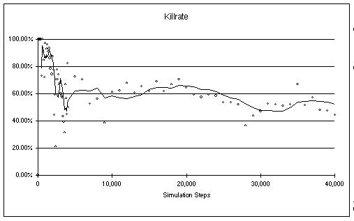
Three phases can be observed. The first phase is the random phase. This
means that the current population consists mainly of creatures which randomly
generated nets. They are usually very badly adapted and die quickly. The
kill rate of this phase is almost 100%. In the above diagram the random
phase lasts for about the first 500 steps of the simulation. If by chance,
two of the randomly created creatures have the capability to survive long
enough, the learning phase is entered. In the learning phase almost no
more random creatures are produced. New creatures are the result of the
above described genetic algorithm. The learning phase in the above diagram
continues from step 500 to about step 5000. I presume that in the learning
phase crossover is the most important operation for the development of
the nets. The so called stable phase follows the learning phase. In this
phase the population has reached its maximum fitness. In our example simulation
the kill rate fluctuates between 60% and 30%. The final kill rate does
not say a lot about the absolute fitness of Nepros as it is strongly dependant
on the density of obstacles. In this phase it is probably mutation that
causes the oscillation of the kill rate. Even if you simulate for a long
time, the fitness of creatures never gets much better than after the learning
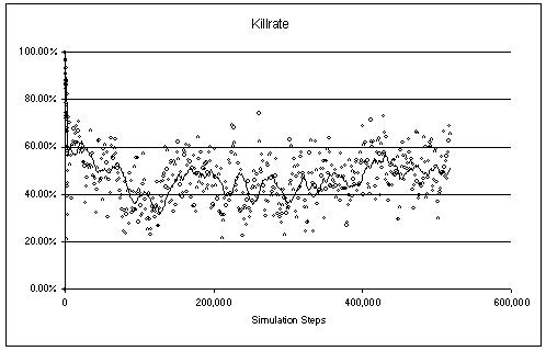
phase. The following diagram shows the same simulation as the one above
but on a different time scale.
Future Work
The exploration of the above described algorithms and its simulation lead
to various questions that could be answered by exploring the results in
more detail or by adding new concepts.
One interesting parameter of evolution is the genetic diversity within
the population. At the moment I can only guess that the diversity is high
in the random phase, decreasing in the learning phase and small in the
stable phase. After exploring the diversity it would be interesting to
explore how the diversity could be influenced and what effects could be
produced by artificially increasing it. Two or more populations could develop
independent of each other. Mixing these populations after a while could
result in fitter creatures.
Another interesting field of research could be the ANN itself. In our
simulation the most simple net was used. It can only react to the current
state of the simulation but does not know anything of the past. So it cannot
make any assumptions about the movements of other objects. The easiest
extension would be to not only feed the current state of the environment
into a creatures net, but to somehow remembered previous states and feed
these together with the current state into the net. This would give the
net the possibility of interpolating from the past to the future and, by
this means (perhaps) react in a better way.
How would recurrent nets behave in our simulation?
What if the genetic algorithm not only changes the weights of the neurons
but also optimizes the topology of the net?
Another nice idea would be to also add "intelligence" to obstacles.
This would extend the simulation to a predator-prey behavior.
I am sure that anyone who tries fiddling with the simulation (changing
parameters and watching what happens) would find lots of open questions
or come up with ideas that would be worthwhile answering or trying out.
But who has the time.
Conclusion
The implementation of the above described algorithm has proved that neuro-evolution
using the above described GA and ANN leads to creatures / robots that adapt
to their environment in a very short time. The behavior is not excellent
in the since that robots do not avoid obstacles 100% of the time, but it
generates stable populations that can survive for a long time.
It seems as if the genetic algorithm does not optimize the individual
creatures / robots but rather searches for an optimal population. Like
in real life, this optimal population does not consist of a collection
of optimal individuals.
References
[Ri94] Rigoll Gerhard; Neuronale Netze. Eine Einführung
für Ingeneure; Informatiker und Naturwissenschaftler; Renninger-Malmsheim:
Expert-Verlag 1994.
[Go89] Goldberg; Genetic Algorithms in Search Optimization
and Machine Learning; Addison-Wesley._
Links
The Nepros Homepage
Neural
Nets Research Groups
The Oberon Homepage
(V4)
Thanks to
Ed and Walter who helped me a lot with this article.